
In the part one about fractional GPUs, we talked about time slicing as "carpooling" for your GPU – getting more people (processes) into the same car (GPU) to use it more efficiently. In this second strategy, called multi-instance GPU (MIG) partitioning, imagine that for the same "carpooling" we get numbered and sized seats for each person so everyone knows where to sit and where they fit. This approach allows for dividing GPUs into isolated and static instances for concurrent usage by different applications.
There is a set of assumptions for the development of this article:
- The experiments and configurations are applied to a Red Hat OpenShift 4.15 cluster
- The GPU used for the experiments is an NVIDIA A100 40GB PCIe
- The software stack deployed to run the experiments is Red Hat OpenShift AI 2.11 with the latest version of the NVIDIA GPU operator
- OpenShift AI v2.X is used to serve models from the flan-t5 large language model (LLM) family
Here we will look at MIG partitioning, how it is configured and how the models behave when doing inference.
What is multi-instance GPU partitioning?
MIG is a feature introduced by NVIDIA that enables a single physical GPU to be split into multiple independent instances. Each instance operates with its own memory, cache and compute cores, effectively allowing different workloads to run concurrently on separate GPU partitions. This is particularly useful for organizations needing to maximize GPU utilization across varied applications without interference.
Advantages of MIG partitioning
- Isolation and enhanced security: Each GPU instance is isolated from the others, so one workload cannot affect the performance or stability of another. This isolation is crucial for running mixed workloads with different priorities and resource requirements
- Resource efficiency: By partitioning the GPU, smaller workloads that do not require the full capability of a high-end GPU can run efficiently, making better use of the available resources. This is ideal for environments with diverse workload sizes
- Scalability: MIG enables scaling by adding more instances to accommodate additional workloads without needing to provision additional physical GPUs. This can significantly reduce costs and improve resource management
On OpenShift, MIG support is provided by the NVIDIA GPU operator. It was developed in cooperation between NVIDIA and Red Hat. Learn how to configure it on the NVIDIA documentation website.
Understanding the GPU geometry
The geometry of a GPU partitioned with MIG involves dividing the GPU into smaller, isolated instances. The partition sizes available depend on the GPU architecture and the driver version being used. For instance, the NVIDIA A100 40GB, offers multiple partitioning options:
- 1g.5gb: 1 Compute Instance (CI), 5GB memory
- 2g.10gb: 2 CIs, 10GB memory
- 3g.20gb: 3 CIs, 20GB memory
- 4g.20gb: 4 CIs, 20GB memory
- 7g.40gb: 7 CIs, 40GB memory
Each partition has its own dedicated set of resources like VRAM, memory bandwidth and compute resources, establishing isolation and preventing interference between workloads.
Partition sizes and driver versions
The availability and configuration of MIG partition sizes can vary depending on the GPU driver version. NVIDIA regularly updates its drivers to support new features, optimizations and partitioning schemes. Here’s an overview of how driver versions might influence MIG partitioning:
- Driver compatibility: Verify that the driver version supports MIG for your specific GPU model. For instance, MIG support for A100 GPUs was introduced in the NVIDIA driver version 450 and above
- Partition flexibility: Newer driver versions might offer enhanced flexibility in creating and managing MIG partitions. For example, additional partition profiles or improved resource allocation algorithms might be available
- Performance improvements: Driver updates often include performance improvements that can affect how MIG partitions behave. This might include better handling of concurrent workloads or more efficient memory management
Configuring the NVIDIA GPU operator
Similar to how it was configured to use time-slicing in the first part of this series of articles, we will use a Kubernetes device plugin as the interface to apply the configuration changes in the nodes containing GPUs.
First, get the current enabled profiles:
oc rsh \
 -n nvidia-gpu-operator \
 $(kubectl get pods -n nvidia-gpu-operator | grep -E 'nvidia-dcgm-exporter.*' | awk '{print $1}') nvidia-smi mig -lgip
The following are the available profiles for MIG partitioning on the NVIDIA A100 GPU, detailing memory allocation, compute units and the maximum number of homogeneous instances:
- 1g.5gb: This profile allocates 5 GB of memory and 1 compute unit, supporting a maximum of 7 homogeneous instances
- 2g.10gb: This profile allocates 10 GB of memory and 2 compute units, allowing for up to 3 homogeneous instances
- 3g.20gb: This profile allocates 20 GB of memory and 3 compute units, with a maximum of 2 homogeneous instances
- 4g.20gb: This profile also allocates 20 GB of memory but with 4 compute units, supporting only 1 homogeneous instance
- 7g.40gb: This profile allocates 40 GB of memory and 7 compute units, and it supports 1 homogeneous instance
It is also possible to use different partition sizes in a mixed-scenario offering flexibility and efficiency by allowing different applications or workloads to use precisely the amount of GPU resources they need.
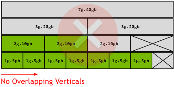
Figure 1. A100 40GB partition geometry
Figure 1 shows how partitions can be configured from the official NVIDIA documentation. Each row describes the maximum amount of partitions of a given size that can be configured in a single GPU. Then they can be configured in a mixed-scenario where you can pick partitions from different rows with the only condition of not having them overlapped in the same column. For example, a valid configuration could be a set of 1g.5g, 1g.5g, 2g.10gb and 3g.20gb MIG partitions.
Enabling MIG partitioning
For this article we will use the simplest configuration approach, which is an homogeneous configuration across all the GPUs in the same node.
NODE_NAME=my-cluster-node.example.com
# MIG_CONFIGURATION=all-1g.5gb
# MIG_CONFIGURATION=all-2g.10gb
# MIG_CONFIGURATION=all-4g.20gb
MIG_CONFIGURATION=all-3g.20gb
# MIG_CONFIGURATION=all-7g.40gb
oc label \
 node/$NODE_NAME \
 nvidia.com/mig.config=$MIG_CONFIGURATION --overwrite=true
With the node labeled we get the enabled devices.
oc rsh \
 -n nvidia-gpu-operator \
$(kubectl get pods -n nvidia-gpu-operator | grep -E 'nvidia-driver-daemonset.*' | awk '{print $1}') nvidia-smi mig -lgi
Which should look like:
+-------------------------------------------------------+
| GPU instances:                                        |
| GPU   Name             Profile  Instance   Placement  |
|                          ID       ID       Start:Size |
|=======================================================|
|   0  MIG 3g.20gb          9        1          4:4     |
+-------------------------------------------------------+
|   0  MIG 3g.20gb          9        2          0:4     |
+-------------------------------------------------------+
In this case, we have two partitions created correctly and we can start working with our experiments for testing MIG behavior.
Performance evaluation of MIG partitioning
The methodology for testing how MIG partitions behave will follow a similar approach we used in our previous article. We will be using Red Hat’s Performance and Scale (PSAP) team’s llm-load-test for benchmarking the performance of LLMs.
Configuring llm-load-test
In this experiment we will measure the throughput and latency of an LLM as the number of parallel queries increases. We query an OpenShift AI inference service endpoint (TGIS standalone), where an LLM from the flan-t5 family (flan-t5-base) was loaded. Once OpenShift AI has been installed and the inference service is up and running, we should get a valid URL where we can ask the model for inference.
To configure llm-load-test, follow the instructions from the first article. For these MIG partitioning experiments, we use a mix of:
- Concurrency: 1, 2, 4, 8, 16, 32 and 64 virtual users. This is the number of parallel queries llm-load-test will run against the API endpoint
- Duration: 100 seconds. This is the time when llm-load-test will run
- Use tls: True. This is to make sure that we will query a TLS endpoint
- Max sequence tokens: 480. This is the total maximum number of tokens from both the input and the output when querying the endpoint
- Max input tokens: 200. This is the maximum number of tokens in the input when querying the endpoint
The results will focus on getting the throughput, time-per-output-tokens (TPOT, percentile 95) and the concurrency values for each test to show how flan-t5-base behaves.
Evaluating LLM results from llm-load-test using MIG partitions
To describe the results we will showcase throughput (x-axis), with respect to the time-per-output-tokens (y-axis), over the different amounts of virtual users used in llm-load-test to query the endpoints.
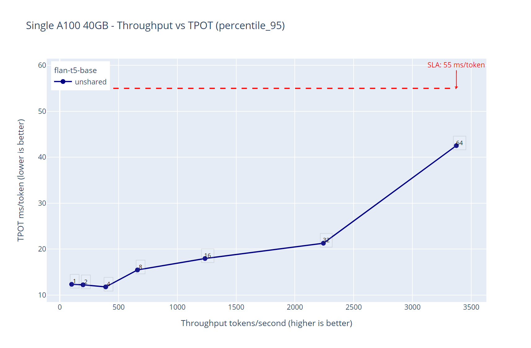
Figure 2. Unshared GPU - flan-t5-base throughput over time-per-output-token latency
Figure 2 shows that the inference service having flan-t5-base was running effortlessly over the maximum of the 64 virtual users used in this experiment, this is expected because this LLM is small, and the GPU capabilities are more than enough to host this small LLM. The maximum throughput is around 3400 tokens per second and the P95 time per output tokens latency was always under our SLA threshold of 55ms.
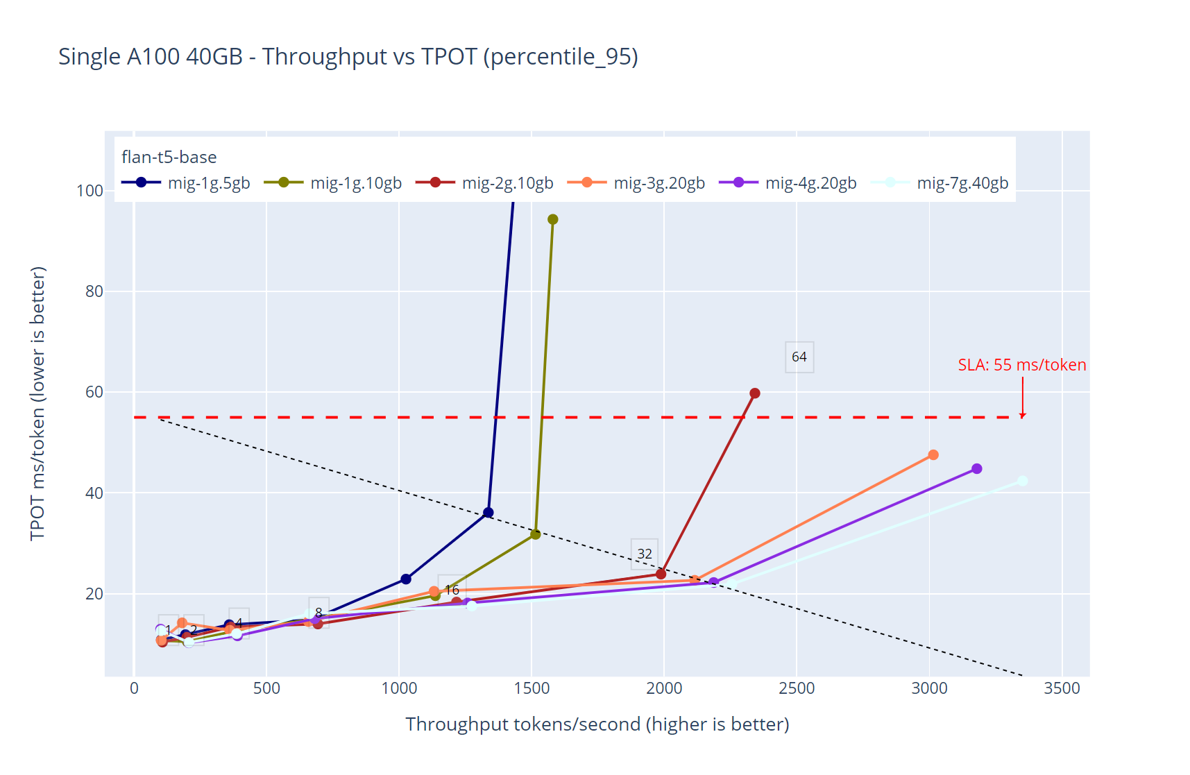
Figure 3. Multiple GPU partition sizes shared with MIG - flan-t5-base throughput over time-per-output-token latency with a single replica
Figure 3 shows an interesting property of how MIG partitions behave. Given that they simulate physical partitions of the GPU, it is expected that bigger partitions (more VRAM, more compute and more memory bandwidth) outperform smaller partitions. We selected flan-t5-base in particular because it is a model that can fit all the current partition sizes available in an A100 40GB GPU.
It is clear that the smaller partition (mig-1g.5gb) behaves ‘slower’ than the biggest partition available (mig-7g.40gb) given its actual capacity capabilities. We also have data points for all the intermediate partition sizes in between (mig-1g.10gb, mig-2g.10gb, mig-3g.20gb and mig-4g.20gb).
This behavior is expected when deploying LLMs using MIG partitions. It is also interesting to note that the latency values spike for single replicas of the predictor pods when the experiment tested over 32 virtual users of concurrency (dashed line denoting 32 concurrent users).
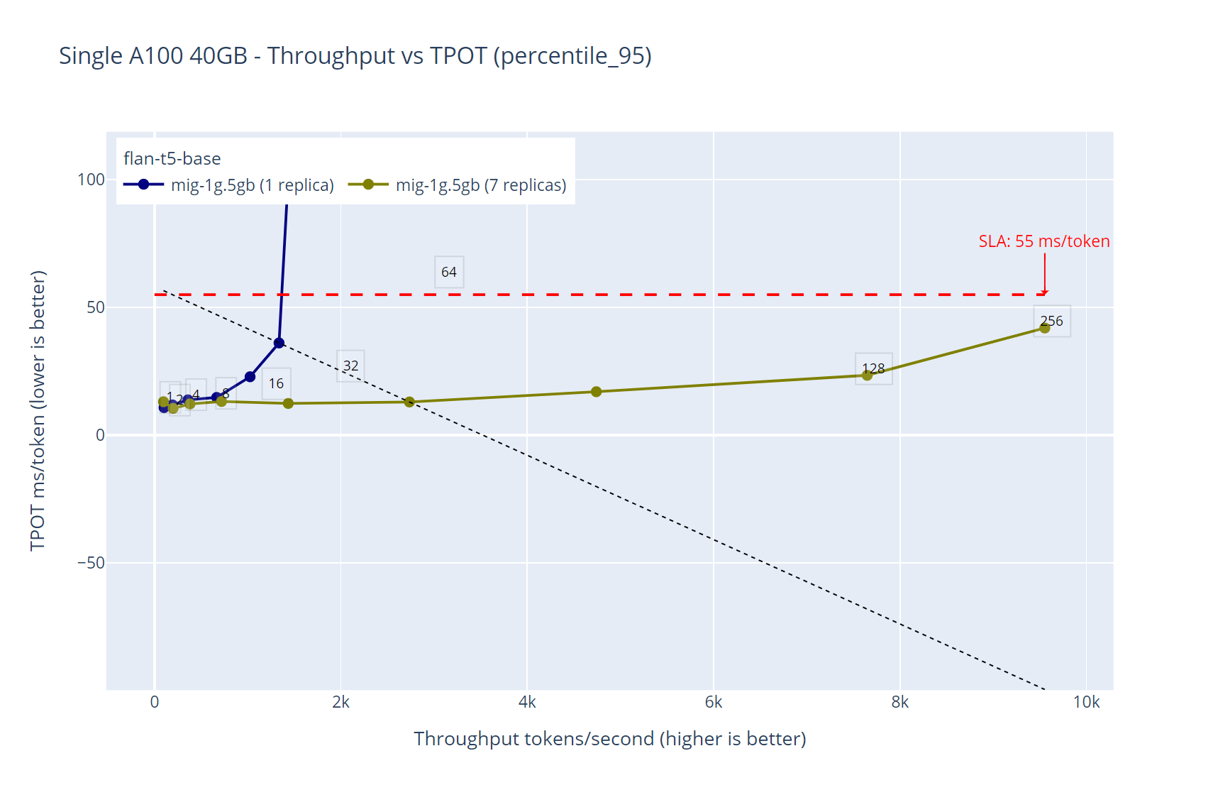
Figure 4. Performance comparison between deploying the same model in a single replica vs the maximum available replicas ‘1g.5gb’ - flan-t5-base throughput over time-per-output-token
An interesting characteristic of the simplest way LLMs can be deployed is that they are stateless and each model that will be tested must be loaded in the GPU VRAM.
Figure 4 shows that we know the workloads that will be deployed. We can maximize the usage of our hardware resources by simply increasing the amount of the predictor pods from the same inference service API endpoint.
In this case, given that the maximum amount of 1g.5g replicas is 7 (for an A100 40GB) we will deploy flan-t5-base 7 times and use the same API endpoint for our tests. The results in figure 4 are self-explanatory—the more replicas we add to the inference service, the bigger is the throughput while keeping the latency under the expected SLA.

Figure 5. Performance comparison between deploying the same model in a single replica vs the maximum available replicas ‘3g.20gb’ - flan-t5-base throughput over time-per-output-token
There is an even more interesting property we can see with more detail in figure 5. This experiment uses a bigger partition size ‘3g.20’ where the maximum number of replicas is 2.
In this case, we can see that the throughput increases linearly with respect to the number of replicas. In this particular example the throughput of a single 3g.20gb partition for 32 virtual users is roughly 2200 tokens per second (blue line), which matches the throughput of roughly 4350 tokens per second using two replicas and 64 virtual users, with all these results keeping the ratio of the SLA under the specified 55 milliseconds. It is important to note that this behavior repeated in all the experiments when testing all the different partition sizes and replicas combinations.
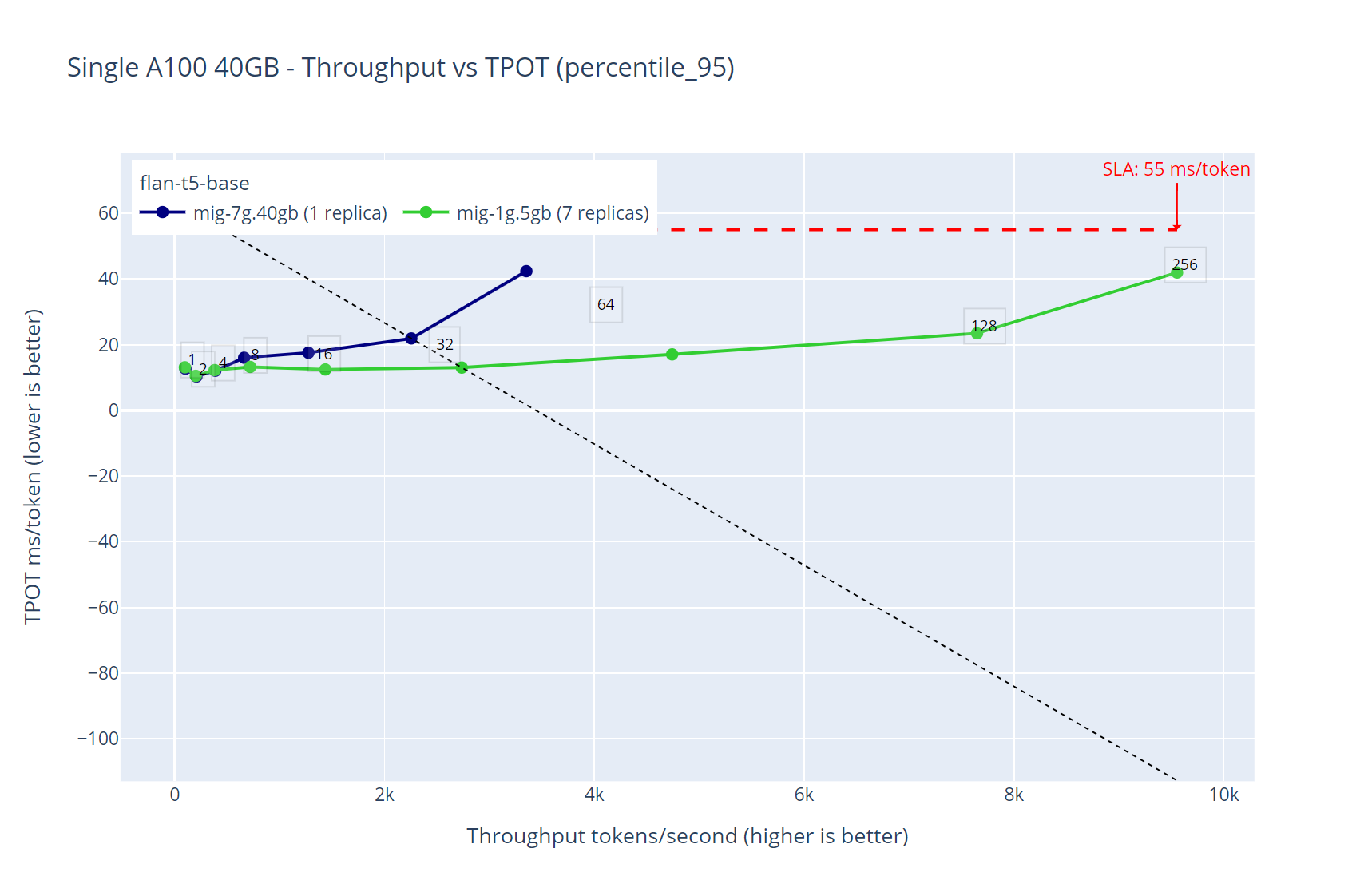
Figure 6. Performance comparison between deploying the same model in a single replica with all the GPU capacity vs the minimum partition size with the maximum available replicas where the model fits - flan-t5-base throughput over time-per-output-token
The results from figure 6 summarizes a potential strategy we can put into practice when there is a need to increase the inference throughput while making sure the inference latency stays under an specific threshold.
If we need to deploy a single model to get the most of our hardware resources it is critical to understand how our workloads behave so we can design our platform to boost its performance.
In this particular case, when deploying the model using the entire GPU, we had a maximum throughput of 4200 tokens per second with a maximum of 64 virtual users. When deploying the same model in the maximum available replicas where it can be loaded, we measured around 9800 tokens per second with a capacity of 256 virtual users, while keeping the latency under our 55ms SLA.
Just like we showed in the first article on using time-slicing as a strategy, this second article on MIG partitioning also demonstrates how critical it is to understand the workloads running to make sure they use all the possible hardware resources.
Some conclusions about the findings when testing MIG partitions.
- MIG offers a robust solution for maximizing GPU utilization, providing isolation, resource efficiency and scalability
- It is particularly beneficial for environments running diverse workloads with varying resource requirements
- Understanding the specific needs of your applications and workloads is crucial to effectively leveraging MIG partitioning
- The availability and configuration of MIG partition sizes can vary depending on the GPU driver version and vendor capabilities
- Bigger partitions outperform smaller partitions
- Multiple smaller partitions might outperform a single bigger partition
À propos des auteurs

Carlos Camacho received the B.Sc. degree in computer sciences from the Central University of Venezuela in 2009, and the M.Sc. and Ph.D. degrees in computer sciences from the Complutense University of Madrid, Spain, in 2012 and 2017, respectively. He received a cum laude mention on his work to formally model Software Product Lines. His research interests include formal methods to model software product lines, distributed systems and cloud computing. He works for Red Hat since 2016, and his current role is Principal Software Engineer part of the Performance and Scale for AI Platforms group.

Kevin Pouget is a Principal Software Engineer at Red Hat on the Performance and Scale for AI Platforms team. His daily work involves designing and running scale tests with hundreds of users, and analysing and troubleshooting how the test enrolled. He has a PhD from the University of Grenoble, France, where he studied interactive debugging of many-core embedded system. Since then, he enjoyed working on different topics around reproducible testing and benchmarking, and finding ways to better understand software execution.

Will McGrath is a senior principal product marketing manager for Red Hat’s AI/ML cloud service, database access service, and other cloud data services on Red Hat OpenShift. He has more than 30 years of experience in the IT industry. Before Red Hat, Will worked for 12 years as strategic alliances manager for media and entertainment technology partners.

Red Hat Performance and Scale Engineering pushes Red Hat products to their limits. Every day we strive to reach greater performance for our customer workloads and scale the products to new levels. Our performance engineers benchmark configurations that range from far edge telco use cases to large scale cloud environments.
We work closely with developers early in the development process to validate that their software design will perform and scale well. We also collaborate with hardware and software partners to ensure that our software is performing and scaling well with their technology, and we engage with customers on innovative deployments where we can apply our expertise to help them get the best performance and scale for their workloads.
We work across the Red Hat product portfolio on a multitude of product configurations and use cases for large scale hybrid cloud environments—including edge-enabled solutions and products, next-generation 5G networks, software-defined vehicles and more.
Contenu similaire
Parcourir par canal

Automatisation
Les dernières nouveautés en matière d'automatisation informatique pour les technologies, les équipes et les environnements

Intelligence artificielle
Actualité sur les plateformes qui permettent aux clients d'exécuter des charges de travail d'IA sur tout type d'environnement

Cloud hybride ouvert
Découvrez comment créer un avenir flexible grâce au cloud hybride

Sécurité
Les dernières actualités sur la façon dont nous réduisons les risques dans tous les environnements et technologies

Edge computing
Actualité sur les plateformes qui simplifient les opérations en périphérie

Infrastructure
Les dernières nouveautés sur la plateforme Linux d'entreprise leader au monde

Applications
À l’intérieur de nos solutions aux défis d’application les plus difficiles

Programmes originaux
Histoires passionnantes de créateurs et de leaders de technologies d'entreprise
Produits
- Red Hat Enterprise Linux
- Red Hat OpenShift
- Red Hat Ansible Automation Platform
- Services cloud
- Voir tous les produits
Outils
- Formation et certification
- Mon compte
- Assistance client
- Ressources développeurs
- Rechercher un partenaire
- Red Hat Ecosystem Catalog
- Calculateur de valeur Red Hat
- Documentation
Essayer, acheter et vendre
Communication
- Contacter le service commercial
- Contactez notre service clientèle
- Contacter le service de formation
- Réseaux sociaux
À propos de Red Hat
Premier éditeur mondial de solutions Open Source pour les entreprises, nous fournissons des technologies Linux, cloud, de conteneurs et Kubernetes. Nous proposons des solutions stables qui aident les entreprises à jongler avec les divers environnements et plateformes, du cœur du datacenter à la périphérie du réseau.
Sélectionner une langue
Red Hat legal and privacy links
- À propos de Red Hat
- Carrières
- Événements
- Bureaux
- Contacter Red Hat
- Lire le blog Red Hat
- Diversité, équité et inclusion
- Cool Stuff Store
- Red Hat Summit