Sharing is caring: How to make the most of your GPUs (part 1 - time-slicing)

As artificial intelligence (AI) applications continue to advance, organizations often face a common dilemma: a limited supply of powerful graphics processing unit (GPU) resources, coupled with an increasing demand for their utilization. In this article, we'll explore various strategies for optimizing GPU utilization via oversubscription across workloads in Red Hat OpenShift AI clusters. OpenShift AI is an integrated MLOps platform for building, training, deploying and monitoring predictive and generative AI (GenAI) models at scale across hybrid cloud environments.

GPU oversubscription is like "carpooling" for your GPU – you’re getting more people (processes) into the same car (GPU) to use it more efficiently. This approach helps you get more throughput, keeping the overall system latency under specific service level agreements (SLAs), and reducing the time the resources are not used. Of course, there can be some traffic jams (too many processes racing for resources), but with the right strategies, and the understanding of your workloads, you can keep the systems consistently outperforming.

This is a series of articles where we will review the different strategies supported by the NVIDIA GPU operator to oversubscribe the available GPU resources. These strategies are tested in the context of the inference service distributed as part of the latest version of OpenShift AI, Text Generation Inference Service (TGIS).

The mainstream three strategies supported by NVIDIA's GPU Operator to oversubscribe GPUs are:

• Time-slicing: Allowing multiple workloads to share GPUs by alternating execution time
• Multi-instance GPU (MIG) partitioning: dividing GPUs into isolated and static instances for concurrent usage by different applications
• Multi-Process Service (MPS): optimizing the execution of parallel GPU workloads by enabling concurrent kernel execution

There is a set of assumptions for the development of this article:

• The experiments and configurations are applied to an OpenShift 4.15 cluster
• The GPU used for the experiments is an NVIDIA A100 40GB PCIe
• The software stack deployed to run the experiments is Red Hat OpenShift AI 2.9 with the latest version of the NVIDIA GPU operator
• Red Hat OpenShift AI v2.X to serve models from the flan-t5 LLM family

In this first article we will look at time-slicing, how it is configured, how the models behave when doing inference with time-slicing enabled and when you might want to use it.

Time-slicing

The simplest approach for sharing an entire GPU is time-slicing, which is akin to giving each process a turn at using the GPU, with every process scheduled to use the GPU in a round-robin fashion. This method provides access for those slices, but there is no control over how many resources a process can request, leading to potential out-of-memory issues if we don't control or understand the workloads involved.

Configuring the NVIDIA GPU operator

The NVIDIA GPU operator can be configured to use the Kubernetes device plugin to manage GPU resources efficiently within the cluster. The NVIDIA GPU operator streamlines the deployment and management of GPU workloads by automating the setup of the necessary drivers and runtime components. With the Kubernetes device plugin, the operator integrates with Kubernetes’ resource management capabilities, allowing for dynamic allocation and deallocation of GPU resources as needed by the workloads.

The Kubernetes device plugin is the interface used to apply the configuration changes in the nodes containing GPUs. When configuring the NVIDIA GPU operator, the device plugin is responsible for advertising the availability of GPU resources to the Kubernetes API, making sure that these resources can be requested by pods and assigned accordingly. These changes can be applied per node.

Configuring time-slicing

The following custom resource (CR) example defines how we will be sharing the GPU in a config map (this won't have any effect on the cluster at the moment). In the CR we specify the sharing strategy for a specific ‘key’—this key is the GPU model ‘NVIDIA-A100-PCIE-40GB’—and we allocate seven replicas for that resource.

cat << EOF | oc apply -f -
---
apiVersion: v1
kind: ConfigMap
metadata:
 name: time-slicing-config
 namespace: nvidia-gpu-operator
data:
 NVIDIA-A100-PCIE-40GB: |-
   version: v1
   sharing:
     timeSlicing:
       resources:
         - name: nvidia.com/gpu
           replicas: 7
EOF

With the resource created, we need to patch the initial ClusterPolicy from the GPU operator called gpu-cluster-policy. The changes need to be applied to the devicePlugin section.

oc patch clusterpolicy \
   gpu-cluster-policy \
   -n nvidia-gpu-operator \
   --type merge \
   -p '{"spec": {"devicePlugin": {"config": {"name": "time-slicing-config"}}}}'

To make sure the resources are configured correctly, we label a specific node stating that the device-plugin.config should point to the configuration we created in the previous steps. This means also that the configuration can be applied on a per node basis.

oc label \
--overwrite node this-is-your-host-name.example.com \
nvidia.com/device-plugin.config=NVIDIA-A100-PCIE-40GB

After a few minutes, we can see that the GPU operator reconfigured the node to use time-slicing. We can verify that by running:

oc get node \
--selector=nvidia.com/gpu.product=NVIDIA-A100-PCIE-40GB \
-o json | jq '.items[0].status.capacity'

The output should look like:

{
"cpu": "128",
"ephemeral-storage": "3123565732Ki",
"hugepages-1Gi": "0",
"hugepages-2Mi": "0",
"memory": "527845520Ki",
"nvidia.com/gpu": "7",
"pods": "250"
}

That means we have seven slices of the GPU ready to be used, identified as  ‘“nvidia.com/gpu”: “7”’.

Performance evaluation of time-slicing

Now that we configured time slicing, let’s compare the performance of an inference workload when the GPU is used by only one replica (not shared) and when we allocate the GPU to multiple replicas of the same inference service (shared with time-slicing).

What is llm-load-test?

Red Hat’s Performance and Scale (PSAP) team created llm-load-test, a tool for benchmarking the performance of large language models (LLMs). Reproducibility is critical when benchmarking, and llm-load-test helps users evaluate performance, enabling better consistency and reliability for LLMs across different environments. By providing a structured framework for performance testing, llm-load-test enables users to understand how their models behave under various loads, helping to identify potential bottlenecks and areas for optimization.

Configuring llm-load-test

In this experiment we will be measuring the throughput and latency of an LLM as the number of parallel queries increases. We will query an OpenShift AI inference service endpoint (TGIS standalone), where an LLM from the flan-t5 family (flan-t5-base) was loaded. Once OpenShift AI has been installed, and the inference service is up and running, we should get a valid URL where we can ask the model for inference.

The first step is to download the latest version of llm-load-test:

git clone https://github.com/openshift-psap/llm-load-test.git
cd llm-load-test

Once in the root folder of the project we need to adjust the configuration YAML file. The following is an abstract of the example configuration file (config.yaml) with the parameters that will be modified for this article.

dataset:
 file: "datasets/openorca_large_subset_011.jsonl"
 max_queries: 1000
 min_input_tokens: 0
 max_input_tokens: 1024
 max_output_tokens: 256
 max_sequence_tokens: 1024
load_options:
 type: constant #Future options: loadgen, stair-step
 concurrency: 1
 duration: 600
plugin: "tgis_grpc_plugin"
grpc/http
 use_tls: True
 streaming: True
 model_name: "flan-t5-base"
 host: "route.to.host"
 port: 443

In the case of these experiments, we use a mix of:

• Concurrency: 1, 2, 4, 8, 16, 32 and 64 virtual users. This is the number of parallel queries llm-load-test will run against the API endpoint
• Duration: 100 seconds. This is the time where llm-load-test will run
• Use tls: True. This is to make sure that we will query a TLS endpoint
• Max sequence tokens: 480. This is the total maximum number of tokens from both the input and the output when querying the endpoint
• Max input tokens: 200. This is the maximum number of tokens in the input when querying the endpoint

Now we run llm-load-test to get the benchmark results from the endpoint:

python3 load_test.py -c my_custom_config.yaml

Once the tests finish the output should look like:

{
 "results":[],
 "config":{
  "load_options": {
     "concurrency": <value>,
  },
 "summary":{
   "tpot": {
     "percentile_95": <value>,
   },
   "throughput": <value>,
 }
}

Where we will be focusing on getting the throughput, time-per-output-tokens (TPOT, percentile 95), and the concurrency values for each test to show how flan-t5-base behaves.

Evaluating large language models results from llm-load-test

To describe the results we will showcase throughput (x-axis), with respect to the time-per-output-tokens (y-axis), over the different amounts of virtual users used in llm-load-test to query the endpoints.

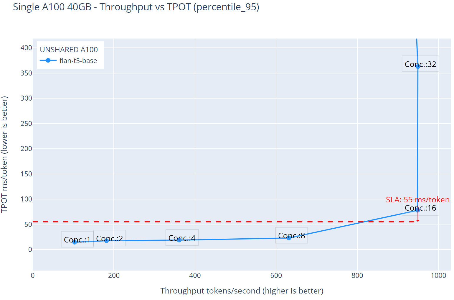
Figure 1. Unshared GPU - flan-t5-base throughput over time-per-output-token latency.

Figure 1 shows that the inference service limit is 16 virtual users, after that, the TPOT latency spikes to values over the boundary SLA of 55 milliseconds per token (this 55ms. boundary ensures that the interaction feels immediate and natural, closely mimicking human conversation, higher values might disrupt the flow of interaction, leading to frustration and a poor user experience). The maximum throughput value is ~980 tokens per second.

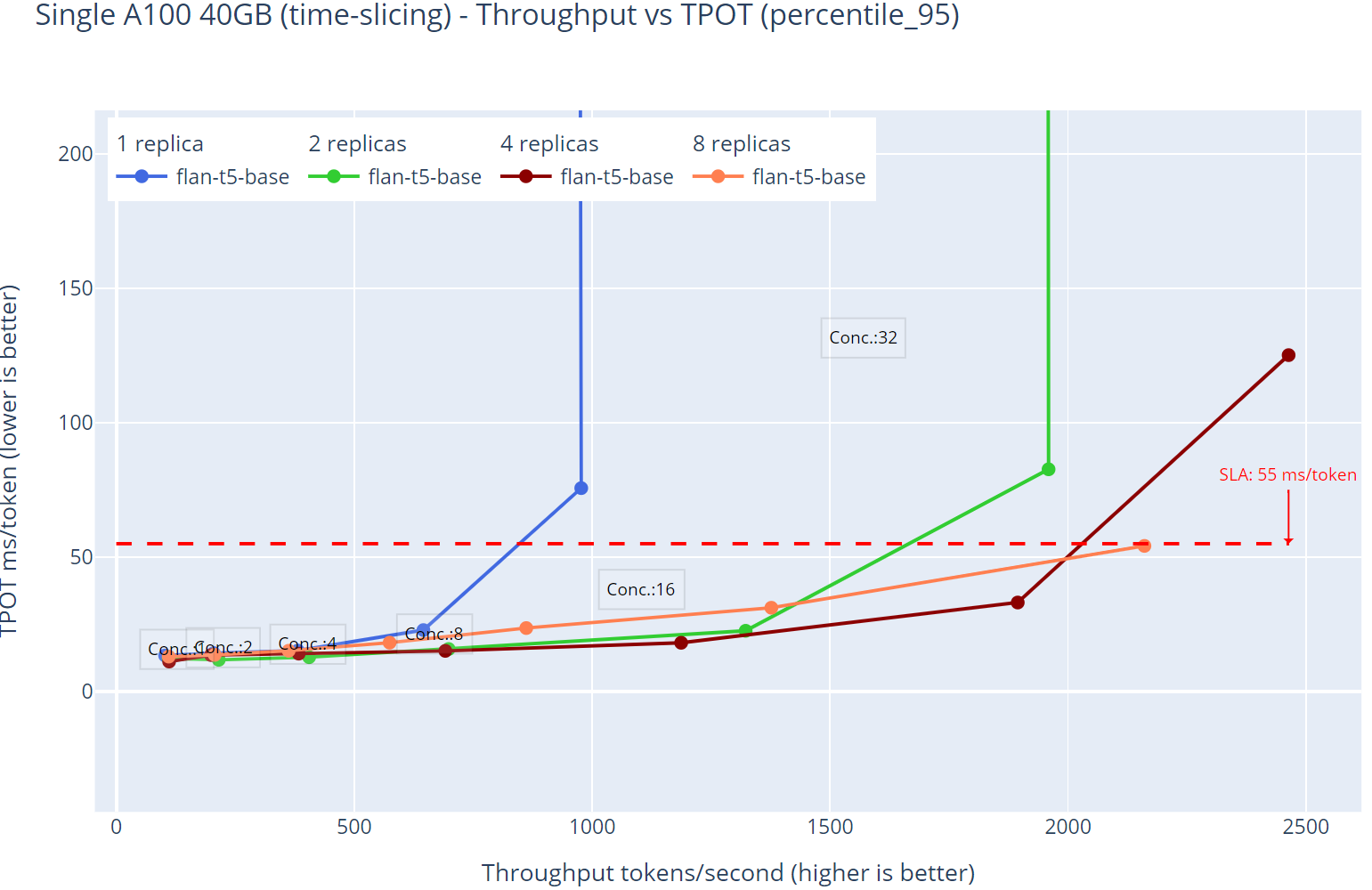
Figure 2. GPU shared with time-slicing - flan-t5-base throughput over time-per-output-token latency with different inference service replicas.

Now let’s introduce time-slicing results. Figure 2 shows different configurations of virtual users, where for 1 and 2 replicas, the inference service latency spikes when the virtual users number is over 16, although the throughput for 2 replicas is ~2000 tokens per second, which is almost twice as many as 1 replica. For the experiments with 4 and 8 replicas of the inference service, we’re able to process 32 and 64 virtual users without the previously described spike in the latency values. There is also an increase in the throughput, but it is not as dramatic as when we compared 1 and 2 replicas from the same inference service. With 8 replicas and 64 virtual users, the load per replica should be ~4 virtual users. This pushes the maximum throughput over 2000 tokens per second without hitting any out-of-memory issues and operates under the SLA of 55 milliseconds.

This small test demonstrates that when sizing the infrastructure to run specific workloads it is crucial to understand the resources they need to run, so you can configure and decide the best strategy to maximize the performance of any application running on the cluster.

Conclusion

When should you use time-slicing as an effective policy for oversubscribing the GPUs?

• When you need to deploy several small models
• When you know how many resources the models will use
• When the workloads are controlled
• When you need a simple configuration to start allocating workloads
• When you're using it for development, testing and staging environments
• When you're using it for workloads without strict latency requirements

In the second part of this series, we will review MIG partitioning, showcasing where it can be useful and the benefits and current drawbacks of that approach.